Graph

Vertex와 Edge로 이루어진 자료구조 G=(V,E)

Undirected graph - Vertex를 잇는 Edge에 방향이 없는 그래프. 최대 edge 수 n(n-1)/2 (n은 vertex개수)

Directed graph - Vertex를 잇는 Edge에 방향이 있는 그래프. 최대 edge 수 n(n-1)

Connected component - 현재 연결성을 유지하면서 더 이상 vertex나 edge를 추가할 수 없는 최대한의 subgraph. connected graph에는 오직 하나의 connected component만이 존재

Cycle - 그래프에서 edge를 통한 순환. cycle은 DFS를 활용해 O(V+E)만에 찾을 수 있음 #

사이클 찾기

그래프는 Adjacency matrix나 Adjacency List (linked adjacency list, array adjancecy list)로 구현

Adjacency matrix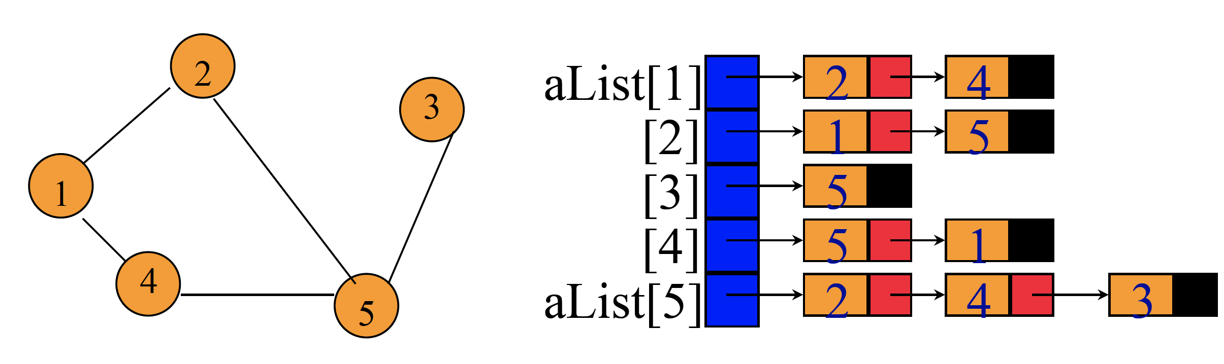

Linked Adjacency List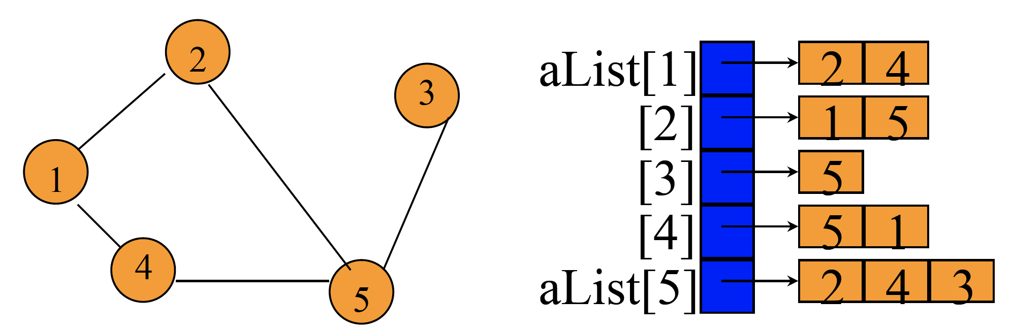

Array Adjacency List

---

Graph search methos (reachable, spanning tree)

DFS(Depth First Search)

dfs(v)
{
	Label vertex v as reached.
	for (each unreached vertex u adjacenct from v)
		dfs(u);
}

u에서 v로 가는 path 찾기: Adjacency matrix 사용시 O(n^2), Adjacency list 사용시 O(n+e)

Connected인지 알아보기: Adjacency matrix 사용시 O(n^2), Adjacency list 사용시 O(n+e)

Spanning tree 만들기: Adjacency matrix 사용시 O(n^2), Adjacency list 사용시 O(n+e)

 

BFS(Breadth First Search)

bfs(v)
{
	Queue q;
    q.enqueue(v);
    record v is visited;
    while(!q.empth())
    {
    	v = queue.front();
        queue.pop();
        if(v is goal)
        	return v;
        for(all vertexes connected with v and not visited)
        {
        	record next_v is visited;
            q.enqueue(next_v);
        }
    }
}

시간복잡도: Adjacency matrix 사용시 O(mn) (m은 component 내의 검색된 vertex의 수), Adjacency list 사용시 O(n + 

number of edges in component)

---

Minimum Spanning Tree

Graph에서 cycle없이 가장 낮은 weight를 가진 edge들로 vertex를 구성

 

Kruskal 알고리즘

1. 아무런 edge도 선택되지 않은 상태에서 시작
2. edge를 weight의 오름차순으로 정렬
3. weight가 낮은 edge부터 선택해 나가며 그래프를 만들어감. cycle이 생길 경우 그 edge는 선택하지 않음

Start with an empty set T of edges.
while (E is not empty && |T| != n-1)
{
	Let (u,v) be a least-cost edge in E.
	E = E - {(u,v)}. // delete edge from E
	if ((u,v) does not create a cycle in T)
	Add edge (u,v) to T.
}
if (| T | == n-1) T is a min-cost spanning tree.
else Network has no spanning tree.

시간복잡도는 O(elog(e)) (e는 edge의 수)

구현은 disjoint set 자료구조를 사용함 #

[알고리즘] Kruskal 알고리즘 이란 - Heee's Development Blog

Prim 알고리즘

1. 하나의 vertex를 선택해 시작
2. 다른 vertex에 가는데 비용이 가장 낮아지는 edge를 선택하여 vertex를 추가
3. 이를 모든 vertex가 추가될 때 까지 반복

//Pseudocode from wikipedia
Associate with each vertex v of the graph a number C[v] (the cheapest cost of a connection to v) and an edge E[v] (the edge providing that cheapest connection). To initialize these values, set all values of C[v] to +∞ (or to any number larger than the maximum edge weight) and set each E[v] to a special flag value indicating that there is no edge connecting v to earlier vertices.
Initialize an empty forest F and a set Q of vertices that have not yet been included in F (initially, all vertices).
Repeat the following steps until Q is empty:
	Find and remove a vertex v from Q having the minimum possible value of C[v]
	Add v to F and, if E[v] is not the special flag value, also add E[v] to F
	Loop over the edges vw connecting v to other vertices w. For each such edge, if w still belongs to Q and vw has smaller weight than C[w], perform the following steps:
		Set C[w] to the cost of edge vw
		Set E[w] to point to edge vw.
Return F

시간복잡도는 Adjacency matrix사용시 O(v^2), Min heap과 Adjacency list 사용시 O(elog(v)), Fibonacci heap과 Adjacency list 사용시 O(e + vlog(v))

 

실제 구현은 BFS와 Adjacency list를 활용 #

[알고리즘] MST(3) - 프림 알고리즘 ( Prim's Algorithm )

Sparse graph는 Kruskal이, dense graph는 Prim이 빠름

 

Sollin 알고리즘

1. 모든 vertex가 선택된 상태로 시작 (edge는 없음)
2. 각 component는 다른 component에 연결되는 가장 weight가 작은 edge를 선택
3. 중복 선택된 edge는 제거
4. 모든 component가 연결되어 component가 하나가 되면 끝
5. weight가 같은 edge가 있으면 cycle이 생길 수 있음

//Pseudocode
Input is a connected, weighted and directed graph.
Initialize all vertices as individual components (or sets).
Initialize MST as empty.
While there are more than one components, do following for each component.
	Find the closest weight edge that connects this component to any other component.
    Add this closest edge to MST if not already added.  
 Return MST.

시간복잡도는 O(elog (v))

실제 구현은 disjoint set 자료구조 사용

---

Shortest path problem

Dijkstra 알고리즘 (single source all destination)

1. 모든 vertex를 미방문 상태로 초기화, 모든 vertex까지의 거리를 무한대로 초기화
2. 출발점 vertex를 방문 상태로 설정, 출발점의 거리는 0
3. 출발점에서 인접한 vertex까지의 거리를 기록하고 이 vertex에 오기 바로 직전 vertex또한 기록. 인접한 vertex는 미방문 상태에서 제외
4. 이를 인접한 vertex에서도 반복하는데 기존에 기록된 거리보다 새로운 거리가 짧으면 새로운 거리로 거리를 업데이트 하고 직전 vertex또한 업데이트.
5. 이를 도착지에 다다를때까지 반복하거나 모든 vertex에 대한 거리를 구하고자 한다면 모든 vertex가 미방분상태에서 제외될 때 까지 반복

//Pseudocode from wikipedia using a priority queue
function Dijkstra(Graph, source):
      dist[source] ← 0                           // Initialization

      create vertex priority queue Q

      for each vertex v in Graph:           
          if v ≠ source
              dist[v] ← INFINITY                 // Unknown distance from source to v
          prev[v] ← UNDEFINED                    // Predecessor of v

         Q.add_with_priority(v, dist[v])


     while Q is not empty:                      // The main loop
         u ← Q.extract_min()                    // Remove and return best vertex
         for each neighbor v of u:              // only v that are still in Q
             alt ← dist[u] + length(u, v) 
             if alt < dist[v]
                 dist[v] ← alt
                 prev[v] ← u
                 Q.decrease_priority(v, alt)

     return dist, prev

구현은 priority queue 사용 # 시간복잡도는 O(e + vlog(v))

다익스트라 알고리즘(Dijkstra Algorithm)